Fellgett’s Advantage

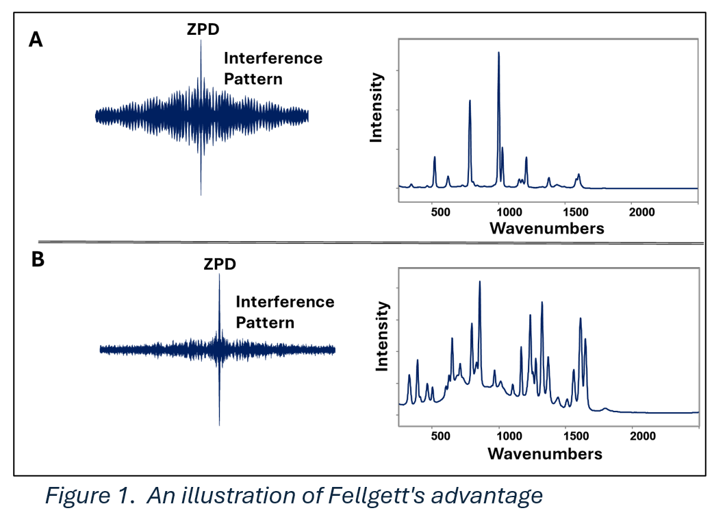
Fellgett’s advantage, also known as the multiplex advantage, arises from how data is distributed in an interferogram. In Figure 1, we illustrate interferogram/spectrum pairs for toluene and acetaminophen. The Zero Path Difference (ZPD) point is where the moving and fixed mirrors of the interferometer are aligned, causing all input frequencies to interfere constructively producing the large central peak in the interferogram.

The advantage appears when the detector has fixed noise, independent of signal intensity. In this case, the high intensity at ZPD leads to low relative noise in the spectrum. For example, acetaminophen, with greater integrated intensity than toluene, exhibits a much larger ZPD peak.

Note that if the detector noise increases with signal intensity (as in shot-noise-limited detectors commonly used in FT-Raman), the benefit may be lost, i.e. a high ZPD intensity may increase noise. In FT-Raman, noise is proportional to the square root of intensity (√I), and the FT algorithm spreads this noise across the spectrum. This can result in baseline noise that exceeds that of a dispersive system.

Jacquinot’s Advantage

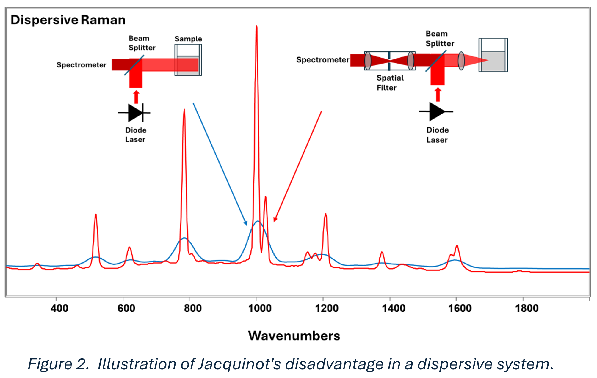
Jacquinot’s advantage is often described as the throughput advantage, but its implications for FT-Raman go far beyond that. In a dispersive Raman system, as shown in Figure 2:

• A large laser spot results in poor resolution and weak signal (blue spectrum).

• Focusing the laser through a spatial filter yields high resolution and better SNR (red spectrum), but samples only a tiny portion of the material.

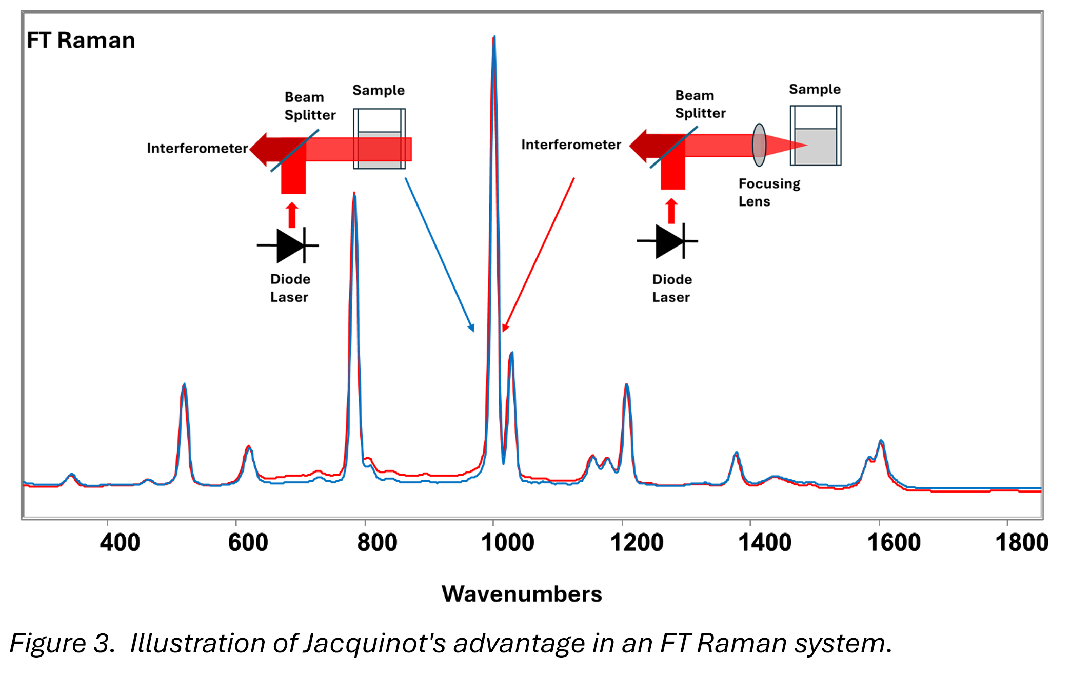
In contrast, Figure 3 shows FT-Raman data collected with an SKM compact instrument:

• Even with a large, unfocused beam, the resolution and signal-to-noise ratio are excellent—this is Jacquinot’s advantage at work.

• A focused beam (right side of Figure 3) gives similar resolution, showing that FT-Raman resolution is independent of beam size.  In FT Raman the spectral resolution is determined by the distance the mirror moves.

Why This Matters:

1. Larger sampling area: A wide laser spot averages over heterogeneous samples, making FT-Raman superior for analyzing real-world materials like illicit drugs or pharmaceutical tablets where composition can vary microscopically.

2. Lower power density: A large beam reduces the laser intensity at the sample. As shown in Figure 4, the unfocused 3 mm beam results in 3600x lower power density than a focused 50 µm beam - greatly minimizing photodamage or sample heating.

Connes’ Advantage

In FTIR spectroscopy, Connes’ advantage refers to the perfect wavenumber calibration enabled using a helium-neon (HeNe) laser as a metrology source. The HeNe laser has a precisely known wavelength, allowing the interferogram to be transformed into a highly accurate wavenumber scale for the FTIR spectrum.

In SKM’s FT Raman system, we apply the same principle but using the Raman excitation laser as the metrology source. This ensures highly precise Raman spectra, delivering the same Connes’ advantage found in FTIR. This level of precision is especially important when building training sets for spectral libraries or large-scale chemometric models, where even small calibration errors can lead to significant analytical issues.

Figure 5 illustrates the benefit of Connes’ advantage in our FT Raman system. The green traces represent the Raman interferogram and its Fourier-transformed spectrum, acquired from the Raman photodetector. The red traces show the metrology interferogram and its spectrum, obtained from a separate photodetector. The metrology spectrum appears as a single sharp peak, defined as 0 wavenumbers, which serves as the anchor for calibrating the Raman spectrum. This precise correlation between the metrology and Raman signals ensures a linear and well-defined wavenumber axis.

This is fundamentally different from dispersive Raman systems, where calibration typically involves measuring reference materials and fitting peak positions to a polynomial function.

Such calibration methods are less precise and more prone to variation over time or between instruments.

Y-Axis (Intensity) Calibration

In addition to precise wavenumber (X-axis) calibration, FT Raman systems offer advantages in Y-axis (intensity) calibration. Dispersive Raman systems require complex Y calibration due to

the wavelength-dependent transfer function of the optical system. This transfer function accounts for:

• Diffraction grating efficiency, which varies with both wavelength and polarization.

• Lens vignetting, where light at the spectral extremes is partially blocked or scattered.

• Optical aberrations, which can distort the focus differently across wavelengths.

• Detector quantum efficiency (QE), which varies across detector elements.

Figure 6 illustrates these effects. The upper section shows how dispersive systems suffer from multiple wavelength-dependent losses—optical and electronic—that combine into a total response function. As a result, each instrument needs its own transfer function correction, often derived from a calibrated white-light source.

In contrast, FT Raman systems are much simpler:

• There are no diffraction gratings or multichannel detectors.

• Only a single photodetector is used, meaning there is no spatial non-uniformity.

• The only necessary Y-axis correction is for the detector's quantum efficiency curve, which is typically provided by the detector manufacturer.

Most importantly, because FT Raman systems lack wavelength-dependent optics and spatially variable detectors, every instrument shares the same calibration structure. This greatly simplifies production, alignment, and data consistency across instruments.  Table 1 provides a comparison of FT Raman and Dispersive Raman calibrations.

Applications Where SKM FT-Raman Excels

• Large chemometric models — Precise, repeatable calibration ensures consistent spectral alignment across instruments.

• High-throughput environments — Minimal calibration downtime, faster instrument swap-out.

• Photosensitive or heterogeneous samples — Jacquinot’s advantage averages power of a large area.

• Field deployment — Compact, stable design with no need for daily recalibration.

• Low-signal Raman — Higher throughput (Jacquinot’s advantage) boosts sensitivity without sacrificing resolution.

Summary

SKM Instruments’ custom compact FT-Raman systems deliver the precision of laboratory-grade FT spectroscopy in a rugged, application-tailored form factor. By combining Connes’ laser-locked calibration, Jacquinot’s high throughput, and optimized Fellgett performance, these instruments outperform dispersive Raman in calibration stability, ease of use, and long-term cost of ownership.

For customers building large spectral libraries, deploying chemometric models, or operating in environments where high laser power density is unacceptable, SKM FT-Raman offers a decisive competitive advantage.

For more information or a pdf version contact us at info@skminst.com.